
If you have lengths stored in inches, like 71.8 for a dining table, you probably want to show them the way people read them: 5′ 11.8″.
Excel has no built-in format or function for this. You build it with a short formula that splits the total into whole feet and leftover inches.
The catch shows up when you round. Many formulas round the inches after the split, so 71.8 inches turns into 5′ 12″ instead of 6′ 0″.
In this article, I’ll show you four ways to convert inches to feet and inches, including a fix for the 5′ 12″ problem and fractions like 11 13/16″.
I’ll also show you how to turn feet and inches back into inches.
Method #1: Using the INT and MOD Functions
This is the simplest way to do it. It works best when your lengths are whole inches, or when you want to keep the decimals as they are.
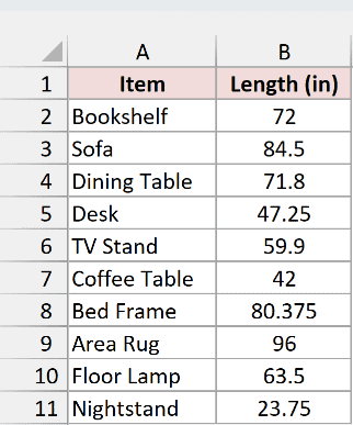
Below I have a dataset with furniture items in column A and their lengths in inches in column B. I want each length in feet and inches.
Here is the formula:
=INT(B2:B11/12)&"' "&MOD(B2:B11,12)&""""
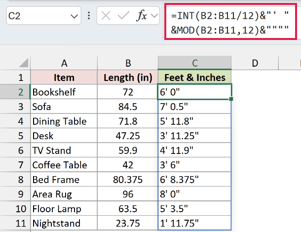
The formula spills down the column automatically in Excel 2021, Excel 2024, and Microsoft 365. In Excel 2019 or older, enter =INT(B2/12)&"' "&MOD(B2,12)&"""" in C2 and copy it down.
How does this formula work?
INT(B2:B11/12) divides each length by 12, and the INT function drops the decimal part, which leaves the whole feet. For 71.8, that’s 5.98, so INT returns 5.
MOD(B2:B11,12) uses the MOD function to return the remainder after dividing by 12. That’s the inches that don’t make up a full foot, which is 11.8 for the dining table.
The & operator joins everything into one text string. "' " adds the foot mark and a space, and """" adds the inch mark.
It takes four quotes because a quote inside a text string has to be typed twice.
Note: Some decimals, like 12.2, can come out as 1′ 0.199999999999999″ because of how Excel stores decimal numbers. To keep up to two decimals without that noise in Excel 2021 or later, use =LET(n,ROUND(B2:B11,2),INT(n/12)&”‘ “&ROUND(MOD(n,12),2)&””””) instead.
Method #2: Using ROUND with INT and MOD
If your lengths have decimals, you’ll often want to round them to the nearest whole inch. This is where most formulas go wrong.
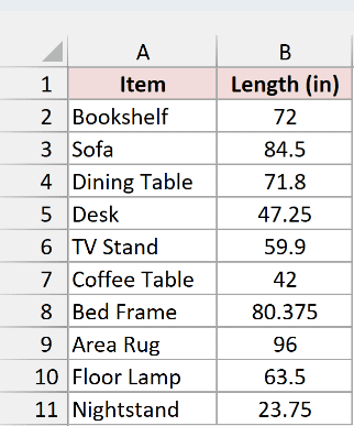
Below I have the same dataset of furniture lengths in inches. I want each length in feet and inches, rounded to the nearest whole inch.
The obvious approach is to wrap the MOD part in ROUND:
=INT(B2:B11/12)&"' "&ROUND(MOD(B2:B11,12),0)&""""
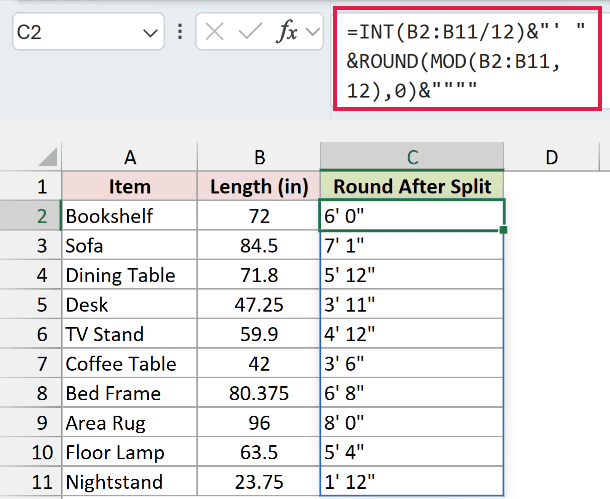
Look at the Dining Table, TV Stand, and Nightstand. They show 5′ 12″, 4′ 12″, and 1′ 12″. Those 12 inches should roll over into the next foot.
This happens because the feet get calculated before the rounding. 71.8 inches is 5 feet and 11.8 inches.
ROUND turns 11.8 into 12, but nothing tells the 5 feet to go up to 6.
The fix is to round the total first and then split it. Here is the formula:
=INT(ROUND(B2:B11,0)/12)&"' "&MOD(ROUND(B2:B11,0),12)&""""
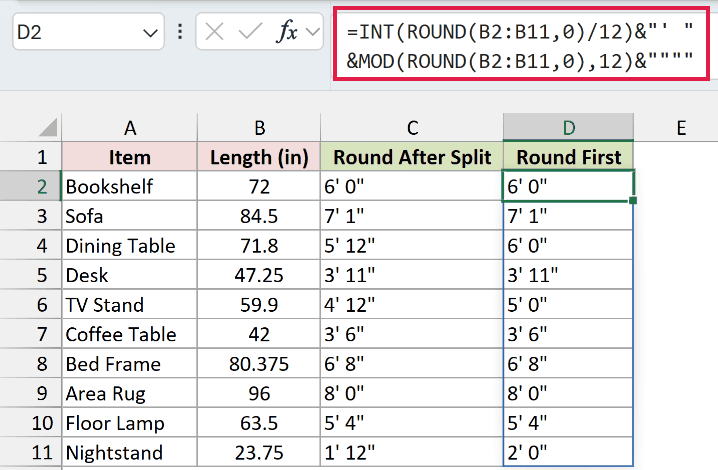
Now the Dining Table shows 6′ 0″, the TV Stand shows 5′ 0″, and the Nightstand shows 2′ 0″.
How does this formula work?
ROUND(B2:B11,0) uses the ROUND function to round each length to the nearest whole inch before anything else happens. 71.8 becomes 72.
INT and MOD then split that rounded number, exactly like in Method #1. 72 divided by 12 is exactly 6 with nothing left over, so you get 6′ 0″.
Because INT and MOD both work on the same rounded value, the feet and inches always agree. This is the version I’d use for most datasets.
Note: To round to the nearest half inch instead, replace ROUND(B2:B11,0) with ROUND(B2:B11*2,0)/2 in both places in the formula.
Method #3: Using the TEXT Function for Fractional Inches
If you work with tape measures or woodworking plans, decimal inches like 11.8″ aren’t much help. You’d rather see 11 13/16″.
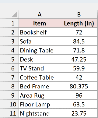
Below I have the same dataset of furniture lengths in inches. I want each length in feet and inches, with fractions rounded to the nearest 1/16 inch.
Here is the formula:
=LET(n,ROUND(B2:B11*16,0)/16,INT(n/12)&"' "&TRIM(TEXT(MOD(n,12),"0 ??/??"))&"""")
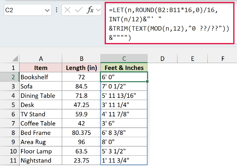
The Dining Table now shows 5′ 11 13/16″, and the Bed Frame shows 6′ 8 3/8″.
How does this formula work?
The LET function lets you calculate a value once, give it a name, and reuse it.
Here the name is n, and it holds each length rounded to the nearest 1/16 inch.
ROUND(B2:B11*16,0)/16 does that rounding. Multiplying by 16 turns inches into sixteenths, ROUND makes that a whole number, and dividing by 16 turns it back into inches. 71.8 becomes 71.8125.
The rounding happens before the split, just like in Method #2, so you never end up with 12 inches.
INT(n/12) returns the feet, and MOD(n,12) returns the leftover inches, which is 11.8125 for the dining table.
The TEXT function with the "0 ??/??" format shows that number as a whole number plus a fraction, so 11.8125 becomes 11 13/16.
Excel also reduces the fraction for you, so 8/16 shows as 1/2.
The 0 in the format keeps a zero when there are no whole inches, so the Sofa shows 7′ 0 1/2″.
TRIM removes the extra spaces TEXT leaves behind when there’s no fraction.
Note: LET works in Excel 2021, Excel 2024, and Microsoft 365. For 1/8 inch precision, change both 16s in the formula to 8.
Method #4: Using INT and MOD in Separate Columns
The first three methods return text. If you still need to do math with the result, put the feet and inches in their own number columns.
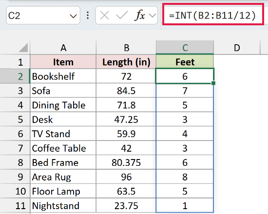
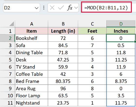
Below I have the same dataset of furniture lengths in inches. I want the feet in column C and the remaining inches in column D.
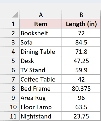
Here is the formula for the feet in cell C2:
=INT(B2:B11/12)
And here is the formula for the inches in cell D2:
=MOD(B2:B11,12)
How do these formulas work?
They use the same math as Method #1, but skip the step that joins everything into text. INT returns the whole feet, and MOD returns the inches left over.
Since both columns hold real numbers, you can sum them, sort by them, or use them in other formulas.
Note: You can still show the foot and inch marks while keeping the numbers. Select column C, press Ctrl + 1 (Cmd + 1 on Mac), and enter 0\’ as a Custom format. Use General\” for column D.
Convert Feet and Inches Back to Inches
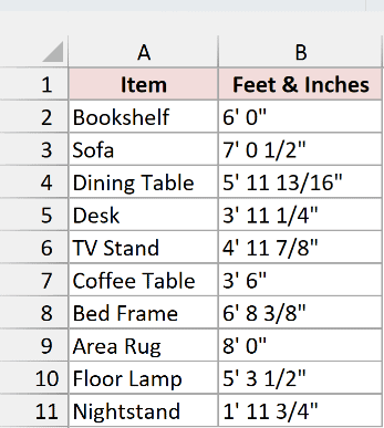
Sometimes you have the opposite problem. Someone sends you a sheet where lengths are already typed as text, like 5′ 11 13/16″, and you need plain inches to calculate with.
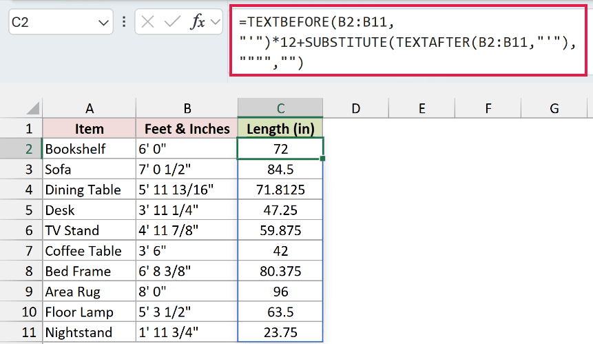
Below I have a dataset with furniture items in column A and lengths as feet-and-inches text in column B. I want the total inches in column C.
Here is the formula:
=TEXTBEFORE(B2:B11,"'")*12+SUBSTITUTE(TEXTAFTER(B2:B11,"'"),"""","")
How does this formula work?
TEXTBEFORE(B2:B11,”‘”) returns everything before the foot mark, which is 5 for the dining table. Multiplying it by 12 turns it into inches and makes Excel treat it as a number.
TEXTAFTER(B2:B11,”‘”) returns everything after the foot mark, which is 11 13/16″. SUBSTITUTE then removes the inch mark, leaving just 11 13/16.
When you add that to the feet, Excel reads 11 13/16 as a mixed fraction. So the dining table comes out as 60 + 11.8125 = 71.8125 inches.
Note: TEXTBEFORE and TEXTAFTER work in Excel 2024 and Microsoft 365. For older versions, there’s a formula in the FAQ below.
Which Method Should You Use?
Here’s how each method handles the same 71.8-inch dining table, so you can pick the one that fits your data.
| Method | Result for 71.8 inches | Best for |
|---|---|---|
| INT and MOD | 5′ 11.8″ | Keeping decimal inches |
| ROUND with INT and MOD | 6′ 0″ | Whole inches (my default) |
| TEXT with fractions | 5′ 11 13/16″ | Tape-measure style lengths |
| INT and MOD in separate columns | 5 and 11.8 | Lengths you still need to calculate with |
Additional Notes About Converting Inches to Feet and Inches in Excel
- The CONVERT function returns decimal feet with
=CONVERT(B2,"in","ft"), so 71.8 comes out as 5.983333. That’s the same as dividing by 12, and it won’t split the result into feet and inches. - Negative lengths break INT and MOD. INT rounds -5.98 down to -6, and MOD returns a positive remainder, so -71.8 comes out as -6 feet and about 0.2 inches. Use
=IF(B2<0,"-","")&INT(ABS(B2)/12)&"' "&MOD(ABS(B2),12)&""""to get -5′ 11.8″. - Methods #1 to #3 return text, so you can’t do math with the results. Text also sorts oddly, so 10′ 2″ comes before 2′ 0″. Keep the original inches column for sums and sorting.
- If you copy lengths from Word or an email, they may use curly marks (’ and ”). The reverse formula only finds the straight ‘ character, so replace the curly ones first.
Frequently Asked Questions
Here are a few questions that come up a lot with this conversion.
How do I show “ft” and “in” instead of the ‘ and ” symbols?
Swap the symbols for words in the formula: =INT(B2/12)&" ft "&MOD(B2,12)&" in". For 71.8 inches, this returns 5 ft 11.8 in.
How do I convert feet and inches back to inches in older versions of Excel?
Use LEFT, FIND, and MID instead of TEXTBEFORE and TEXTAFTER: =LEFT(B2,FIND("'",B2)-1)*12+SUBSTITUTE(MID(B2,FIND("'",B2)+1,99),"""",""). For 5′ 11 13/16″, it returns 71.8125.
How do I convert centimeters to feet and inches in Excel?
Convert to inches with CONVERT first, then split the rounded result: =LET(n,ROUND(CONVERT(B2,"cm","in"),0),INT(n/12)&"' "&MOD(n,12)&""""). For 170 cm, this returns 5′ 7″.
How do I convert decimal feet like 5.75 to feet and inches?
Multiply by 12 to get inches, then use the Method #2 formula: =INT(ROUND(B2*12,0)/12)&"' "&MOD(ROUND(B2*12,0),12)&"""". For 5.75 feet, this returns 5′ 9″.
Conclusion
INT and MOD handle the actual conversion to feet and inches in Excel. The part that trips people up is rounding, so always round the total before you split it.
In this article, I showed you four ways to convert inches to feet and inches, plus a formula to turn them back into inches.
For most lists, I’d go with Method #2.
I hope you found this article helpful.
Other Excel articles you may also like:
