
Excel can handle complex numbers, but it stores them as text. You’ll need its IM functions to calculate with them.
Throughout these examples, I’ll use AC circuit impedance, where the real part represents resistance and the imaginary part represents reactance.
I’ll show you how to create and split complex numbers, do arithmetic, find magnitude and angle, convert between rectangular and polar form, and clean up tiny rounding errors.
How Excel Stores Complex Numbers
You write a complex number in the form a+bi, where a is the real part and b is the imaginary coefficient.
For example, 40+30i has a real part of 40 and an imaginary part of 30. You can use lowercase i or j.
Excel has no complex number data type. Values you type this way, and complex results returned by COMPLEX or IM functions, are text.
The ordinary +, -, *, and / operators won’t work on these complex values, so I’ll use the IM functions.
IMREAL and IMAGINARY pull out the real and imaginary parts. IMABS gives you the size, or magnitude. All three return ordinary numbers.
How to Create Complex Numbers in Excel
You can type the complete value or build it from separate real and imaginary parts.
Method #1: Typing the Complex Number Directly
For a few fixed values, you can enter each complex number directly. Type 40+30i into a cell and press Enter; Excel keeps it as text.
Below I have a dataset of loads and their typed impedances on the Real and Imaginary Parts sheet, in A1:B10.
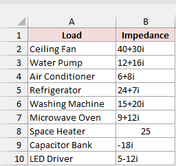
The Ceiling Fan value is 40+30i, while the LED Driver value is 5-12i. A negative imaginary part uses a minus sign.
This works when your values won’t change, but it’s easy to mistype a sign. A typed value won’t update when your resistance or reactance changes.
Method #2: Using the COMPLEX Function
When your real and imaginary parts already sit in separate columns, I recommend using COMPLEX. You can change either input and the result updates.
Below I have a dataset on the Create Complex Numbers sheet, with loads in column A, resistance in B, and reactance in C.
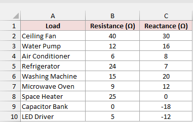
Enter this formula in D2 and copy it down to D10.
The IM functions and COMPLEX don’t spill when you pass them a whole range, so you’ll need one formula per row.
=COMPLEX(B2,C2)
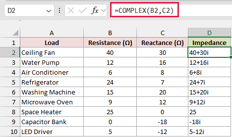
How does this formula work?
COMPLEX joins the resistance in B2 with the reactance in C2, returning 40+30i for the Ceiling Fan.
The first argument, real_num, is your real part. The second, i_num, is your imaginary coefficient. An optional third argument chooses the suffix, "i" or "j".
You don’t need to supply that third argument for i, because it’s the default.
COMPLEX leaves out zero parts. The Space Heater returns 25, and the Capacitor Bank returns -18i. Both are still text results from COMPLEX.
How to Get the Real and Imaginary Parts
Once you have a value such as 40+30i, you can pull out its two parts with IMREAL and IMAGINARY.
Below I have a dataset on the Real and Imaginary Parts sheet, with loads in column A and typed impedances in B.
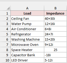
To extract the real part, enter this formula in C2 and copy it down to C10:
=IMREAL(B2)
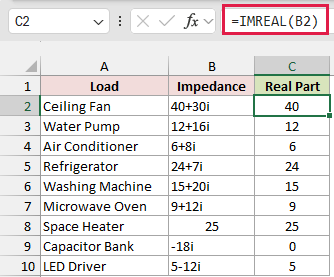
IMREAL reads the complex value in B2 and returns 40. For the Capacitor Bank’s -18i, it returns 0 because there’s no real part.
To extract the imaginary coefficient, enter this formula in D2 and copy it down to D10:
=IMAGINARY(B2)
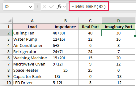
IMAGINARY returns 30 for 40+30i and -12 for 5-12i. You get the coefficient, without the i suffix.
Both functions return ordinary numeric values, so you can use their results in regular Excel calculations.
How to Add, Subtract, Multiply, and Divide Complex Numbers
You can’t use +, -, *, or / directly on complex text. For example, =B2+C2 returns #VALUE! when both cells contain complex numbers.
Below I have a dataset on the Arithmetic sheet, with circuits in A and two load impedances in B and C, across rows 2:7.
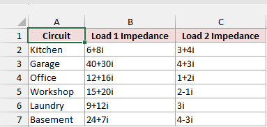
I’ll use a separate IM function for each operation, starting with addition. Enter this formula in D2 and copy it down to D7:
=IMSUM(B2,C2)
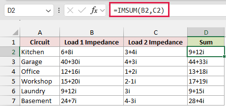
IMSUM adds the real parts together and the imaginary parts together. For Kitchen, 6+8i plus 3+4i returns 9+12i.
To subtract Load 2 from Load 1, enter this formula in E2 and copy it down to E7:
=IMSUB(B2,C2)
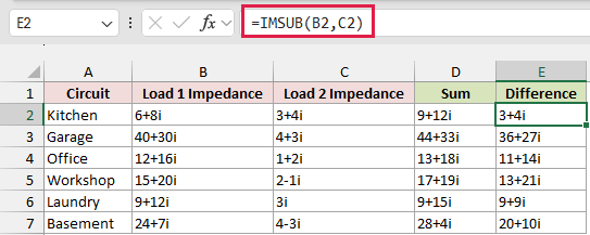
IMSUB subtracts the second value from the first. For Kitchen, the result is 3+4i, so your argument order matters.
To multiply the two values, enter this formula in F2 and copy it down to F7:
=IMPRODUCT(B2,C2)
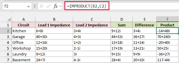
IMPRODUCT returns -14+48i for Kitchen. The real part includes 6*3 - 8*4, because multiplying the two imaginary terms introduces a negative sign.
To divide Load 1 by Load 2, enter this formula in G2 and copy it down to G7:
=IMDIV(B2,C2)
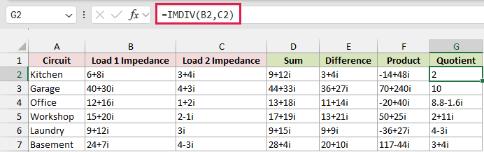
IMDIV divides the first value by the second. Kitchen returns 2, while Office returns 8.8-1.6i.
For Garage, 40+30i divided by 4+3i returns exactly 10, because both parts of Load 1 are ten times those of Load 2.
IMSUB and IMDIV each take exactly two values. Dividing by zero with IMDIV returns #NUM!.
You can also add an entire range with IMSUM, without listing each cell separately.
Below I have a dataset on the Sum a Range sheet, with nine loads in A2:A10 and their impedances in B2:B10.
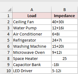
To calculate the total impedance of these loads in series, enter this formula in E1, beside the Total Impedance label in D1:
=IMSUM(B2:B10)
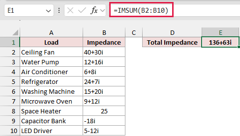
The result is 136+63i. IMSUM combines all nine real parts and all nine imaginary parts into one complex result.
You can give IMPRODUCT a range too, but a blank cell in that range makes it return 0. IMSUM skips blank cells in a referenced range.
How to Find the Magnitude and Angle
A value such as 40+30i describes two components. You can also describe it by its overall size and angle, called polar form.
Below I have a dataset on the Modulus and Angle sheet, with loads in column A and their impedances in B.
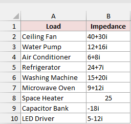
To find the magnitude, enter this formula in C2 and copy it down to C10:
=IMABS(B2)
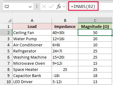
IMABS returns the magnitude, also called the modulus. For the Ceiling Fan’s 40+30i, you get 50 ohms.
That 50 comes from the square root of 40² + 30². The result is an ordinary number you can use in other calculations.
To find the angle, enter this formula in D2 and copy it down to D10:
=IMARGUMENT(B2)
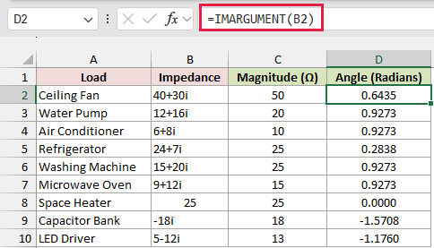
IMARGUMENT returns radians between negative pi and positive pi. The Ceiling Fan’s angle displays as 0.6435, with column D showing four decimal places.
To display the angle in degrees instead, enter this formula in E2 and copy it down to E10:
=DEGREES(IMARGUMENT(B2))
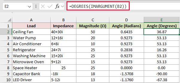
DEGREES converts the angle returned by IMARGUMENT. With column E showing two decimal places, the Ceiling Fan’s angle is 36.87 degrees.
So you can describe 40+30i as 50 ohms at 36.87 degrees. The Capacitor Bank’s -18i has magnitude 18 and angle -90 degrees.
An angle isn’t defined for zero, so IMARGUMENT returns #DIV/0! when you pass it "0".
How to Convert Polar Form to Rectangular Form
When you already have a magnitude and angle, you can calculate the real and imaginary parts, then join them with COMPLEX.
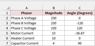
Below I have a dataset on the Polar to Rectangular sheet, with phasors in A, magnitudes in B, and angles in degrees in C.
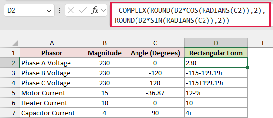
Enter this formula in D2 and copy it down to D7:
=COMPLEX(ROUND(B2*COS(RADIANS(C2)),2),ROUND(B2*SIN(RADIANS(C2)),2))
How does this formula work?
RADIANS converts your angle in C2 from degrees to radians, which is the unit COS and SIN need.
Multiplying the magnitude by COS calculates the real part. Multiplying it by SIN calculates the imaginary coefficient.
ROUND rounds each component to two decimal places before COMPLEX joins them. This keeps long decimals and tiny leftovers out of the final text.
Phase B Voltage, with magnitude 230 and angle -120 degrees, returns -115-199.19i. Motor Current, with magnitude 15 and angle -36.87 degrees, returns 12-9i.
For Capacitor Current, magnitude 4 at 90 degrees returns 4i. Rounding removes the tiny real remainder that can otherwise appear at this angle.
Other Complex Number Functions in Excel
You can also flip the imaginary sign, raise a complex number to a power, or calculate its square root.
Below I have a dataset on the Other Functions sheet, showing those three operations on 3+4i, with formulas in column C and results in D.
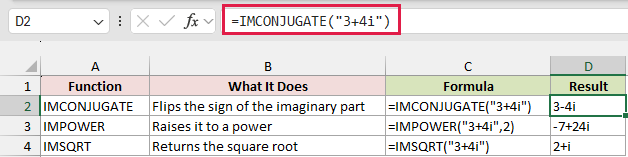
IMCONJUGATE returns 3-4i, changing only the imaginary sign. That flipped version is called the complex conjugate.
IMPOWER with a power of 2 returns -7+24i. IMSQRT returns 2+i. Column C uses FORMULATEXT so you can read each calculation beside its result.
For trigonometric, exponential, and logarithmic calculations, you also have IMSIN, IMCOS, IMTAN, IMEXP, IMLN, IMLOG10, and IMLOG2.
How to Fix Tiny Rounding Errors in Complex Results
Sometimes a result includes a tiny extra component, even when you’d expect that component to be zero.
Below I have a dataset on the Tiny Rounding Errors sheet, with calculations in A and raw complex results in B.
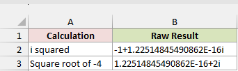
Squaring i returns -1+1.22514845490862E-16i. The square root of -4 returns 1.22514845490862E-16+2i.
That E-16 component is a floating-point leftover, effectively zero at this scale. It doesn’t mean your input data is wrong.
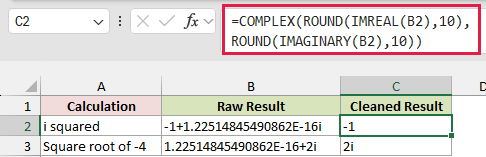
To clean both results, enter this formula in C2 and copy it down to C3:
=COMPLEX(ROUND(IMREAL(B2),10),ROUND(IMAGINARY(B2),10))
How does this formula work?
IMREAL and IMAGINARY extract the two numeric components. ROUND rounds each one to ten decimal places, and COMPLEX rebuilds the complex text.
The cleaned results are -1 and 2i. Choose a rounding precision that fits your calculation, because rounding also removes genuine digits beyond that precision.
Additional Notes About Working With Complex Numbers in Excel
Keep these checks in mind when you work across several complex-number calculations:
- Keep the suffix consistent throughout a calculation. Lowercase
iandjare valid, but mixing them in one IM function can return#VALUE!. - Use IMSUM for complex text instead of SUM, which ignores text in referenced cells. Numeric outputs from IMREAL, IMAGINARY, IMABS, and IMARGUMENT work with SUM normally.
- In Microsoft 365, you can spill per-cell calculations with
=MAP(B2:B10,LAMBDA(z,IMREAL(z))), which applies IMREAL to each value in the range. - Check the input when you see
#NUM!or#VALUE!. A malformed value such as3+4returns#NUM!; an incompatible suffix or calculation can produce#VALUE!. - Keep angle units visible in your column headings. IMARGUMENT returns radians, so label converted degree values separately to avoid using the wrong unit later.
Frequently Asked Questions
Here are a few more questions you may have when working with imaginary numbers in Excel.
Can Excel plot complex numbers?
Yes. Use IMREAL and IMAGINARY to create numeric helper columns, then insert a scatter chart with the real parts on X and imaginary parts on Y.
Do I need the Analysis ToolPak for complex number functions?
No. The complex-number functions are built into current Excel, so you can enter these formulas without enabling the Analysis ToolPak.
How do I write j instead of i in Excel?
Use the third argument of COMPLEX. For example, =COMPLEX(3,4,"j") returns 3+4j. You can also type 3+4j directly into a cell.
Conclusion
I’d start with COMPLEX to build the value, then use IM functions for arithmetic, extracting components, and finding magnitude and angle for polar form.
If you get tiny rounding errors, my cleanup trick is to ROUND the real and imaginary parts separately, then rebuild the value with COMPLEX.
Other Excel articles you may also like:
