New Excel Functions in Microsoft 365 (With Examples)

Excel has picked up a lot of new functions over the last few years. If you only know XLOOKUP and maybe FILTER, you’re missing some really handy ones.

In this article, I’ll walk you through 44 of them. You get one working formula for each, plus a short example that shows what it does.

I’ve grouped them by the job they do, like filtering data, splitting text, or summarizing numbers. That way, you can jump straight to the task you have.

If you’re new to these, start with FILTER. It’s the easiest one to see in action, and it makes the rest of the list a lot easier to follow.

The example file has a sheet for every function, so you can follow along as you read.

Dynamic Array Functions

These formulas return arrays that can spill into neighboring cells. Start with FILTER when you want rows that meet a condition.

FILTER

FILTER pulls out only the rows that match a condition you set.

Think of it as the filter button, except the results show up in a new spot and your original data stays untouched.

The best part is that it updates on its own. Change a value in the source data, and the filtered list changes right away.

It’s great for pulling one region, product, or status from a bigger table.

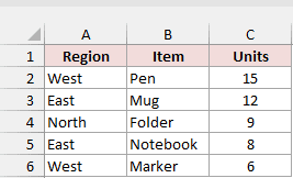
Keep only East-region orders from the five-row source.

=FILTER(A2:C6,A2:A6="East","No matches")

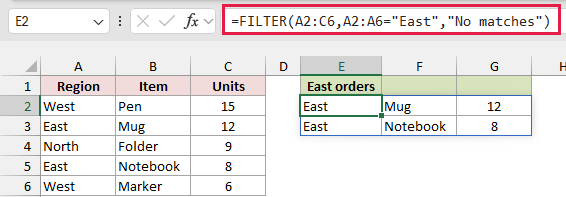
The two East rows spill with their item and unit columns.

SORT

SORT gives you a sorted copy of a range without touching the original. You tell it which column to sort by and whether you want ascending or descending order.

I like it for things like a dashboard or a report sheet, where the raw data should stay as it is but you want a sorted view next to it.

Sort the product list by its second column in ascending order.

=SORT(A2:B6,2,1)

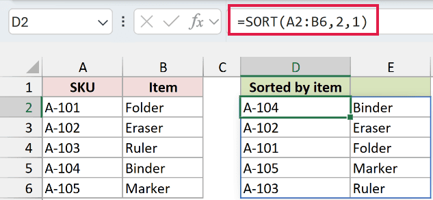
The product rows spill in item-name order.

SORTBY

SORTBY is SORT’s more flexible sibling. It sorts one range based on the values in another range, and that other range doesn’t even need to be part of the result.

It’s handy when you want to sort by more than one column, or show a list of names sorted by sales without showing the sales numbers.

Sort branch rows by their sales values from highest to lowest.

=SORTBY(A2:B6,B2:B6,-1)

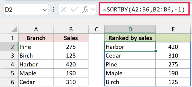
Harbor, the highest-sales branch, appears first.

UNIQUE

UNIQUE gives you each value from a list just once, with all the repeats removed. It’s the formula version of Remove Duplicates, except your original list stays as it is.

You’ll use it all the time for building dropdown lists, counting how many different customers or products you have, or getting a clean list of categories.

Return each drink category once from the source list.

=UNIQUE(A2:A7)

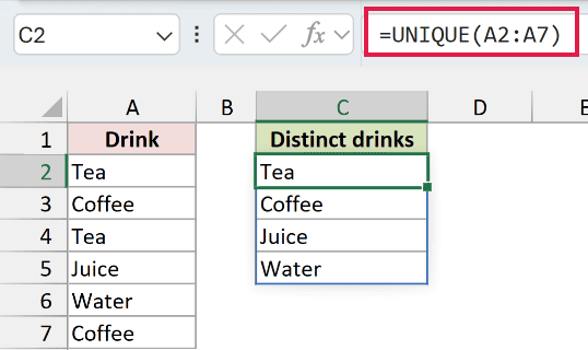
Tea, Coffee, Juice, and Water appear as a distinct list.

SEQUENCE

SEQUENCE creates a list of numbers for you. You pick how many rows and columns you want, where it starts, and how much it goes up by each step.

It’s useful for numbering rows, building a list of dates, or creating a quick grid of values without typing or dragging anything.

Generate five rows and two columns, starting at 10 and increasing by 10.

=SEQUENCE(5,2,10,10)

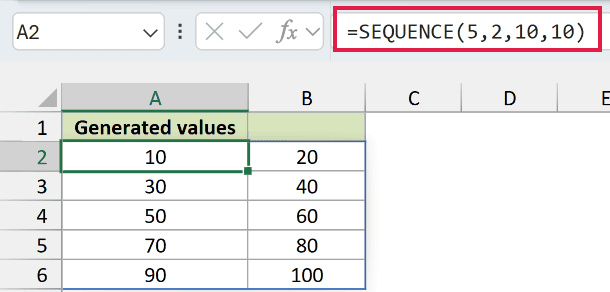
The grid runs from 10 to 100.

RANDARRAY

RANDARRAY fills a range with random numbers. You choose the size, the lowest and highest values, and whether you want whole numbers or decimals.

It’s handy for creating test data or picking random samples.

Just remember the numbers change every time Excel recalculates, so paste them as values if you need them to stay put.

Generate five random whole numbers from 1 through 20.

=RANDARRAY(5,1,1,20,TRUE)

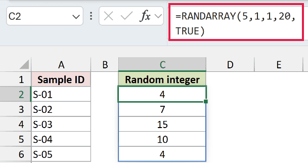
The five results change when Excel recalculates.

Lookup Functions and LET

XLOOKUP and XMATCH find a value or its position. LET lets you name part of a formula so you don’t have to repeat it.

XLOOKUP

XLOOKUP finds a value in one column and returns the matching value from another.

It replaces VLOOKUP and HLOOKUP, and the result column can sit on either side of the lookup column.

You can also set your own message for when nothing matches, so there’s no need to wrap it in IFERROR.

For most lookups today, this is the one I’d reach for.

Find product P-104 in the inventory and return its item name.

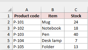
=XLOOKUP("P-104",A2:A6,B2:B6,"Not found")

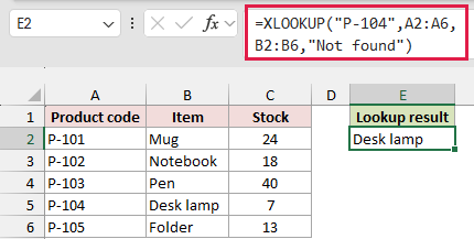
The result is Desk lamp.

XMATCH

XMATCH tells you where a value sits in a list. Instead of returning the value itself, it returns its position, like 4 for the fourth item.

It’s the newer version of MATCH, and it defaults to an exact match, which is what you want most of the time. It also pairs nicely with INDEX.

Find the position of P-104 in the product-code list.

=XMATCH("P-104",A2:A6,0)

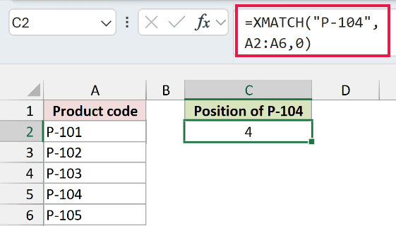
The result is 4.

LET

LET lets you give a name to a value or calculation inside a formula, then use that name as many times as you want.

This makes long formulas easier to read, and Excel works out the named part only once.

If you ever repeat the same chunk several times in one formula, LET is your fix.

Name the total order count, then divide it by the five populated days.

=LET(total,SUM(B2:B6),total/COUNTA(B2:B6))

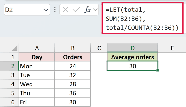
The average is 30 orders.

LAMBDA and Its Helper Functions

LAMBDA defines a calculation. Its helper functions apply a calculation to values, rows, columns, or an entire generated array.

LAMBDA

LAMBDA lets you create your own function using a regular Excel formula. You define the inputs, write the calculation once, and reuse it.

Save it with a name in the Name Manager and you can use it across the whole workbook, just like a built-in function.

It also powers MAP, REDUCE, SCAN, and the rest of this group.

Define a 10% price increase and immediately apply it to B2.

=LAMBDA(price,price*1.1)(B2)

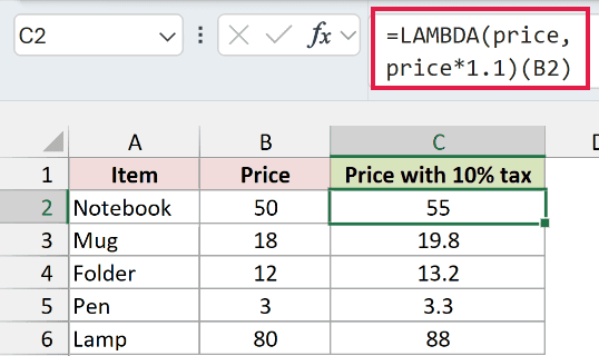
A $50 price becomes $55.

MAP

MAP runs a calculation on every value in a range, one at a time, and gives you back a new range of results.

It really shines when your calculation uses functions like AND, OR, or SUM, which would otherwise collapse the whole range into a single answer.

Apply a 10% increase to each base value.

=MAP(A2:A6,LAMBDA(n,n*1.1))

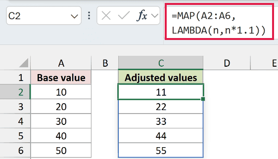
The five adjusted values spill beside the originals.

REDUCE

REDUCE goes through a range one value at a time and keeps a running result, then gives you just the final answer.

Think of it as a custom SUM. You decide what happens at each step, so it can add, multiply, count, or combine values in ways the regular functions can’t.

Accumulate five daily donations into one value.

=REDUCE(0,A2:A6,LAMBDA(total,n,total+n))

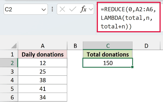
The final total is 150.

SCAN

SCAN works like REDUCE, but it shows you every step along the way instead of just the final answer.

That makes it perfect for running totals, running balances, or any calculation where each row builds on the one before it.

Show the intermediate total after each daily donation.

=SCAN(0,A2:A6,LAMBDA(total,n,total+n))

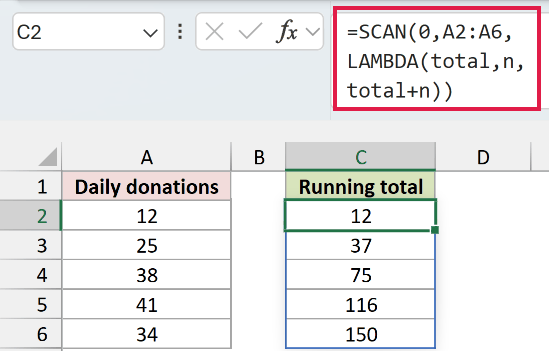
The running totals end at 150.

MAKEARRAY

MAKEARRAY builds a grid of any size you choose. For each cell, it passes the row and column number to a LAMBDA, and the LAMBDA decides what goes there.

It’s great for things like multiplication tables, calendars, or any layout where the value depends on its position.

Build a four-row, three-column multiplication grid from row and column numbers.

=MAKEARRAY(4,3,LAMBDA(r,c,r*c))

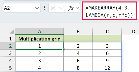
The bottom-right value is 12.

BYROW

BYROW applies a calculation to each row of a range and returns one result per row.

A regular SUM or MAX on a range gives you one number for the whole thing.

BYROW gives you a separate answer for every row, from a single formula that spills down.

Sum each team’s three weekly values.

=BYROW(B2:D6,LAMBDA(row,SUM(row)))

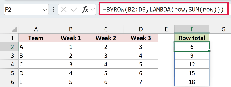
One total spills for each team row.

BYCOL

BYCOL is the column version of BYROW. It runs a calculation on each column of a range and returns one result per column.

Use it for column totals, averages, or the highest value in each column, all from one formula instead of one formula per column.

Sum each day column across the five rows.

=BYCOL(A2:E6,LAMBDA(col,SUM(col)))

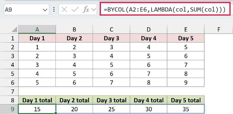
The daily totals spill across columns.

ISOMITTED

ISOMITTED checks whether an argument was left out when your LAMBDA was called. It returns TRUE if the value is missing and FALSE if it was given.

It’s what lets you build custom functions with optional arguments, so you can fall back to a default value when someone skips one.

Test whether an optional argument was supplied to a LAMBDA.

=LAMBDA(value,[alternate],IF(ISOMITTED(alternate),value,alternate))("Confirmed")

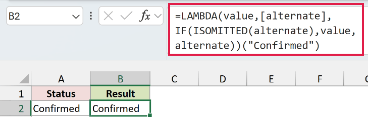
With the optional argument omitted, the result is Confirmed.

Text Functions

These functions turn values into text or separate text at a delimiter. Choose the one that matches the shape you need.

ARRAYTOTEXT

ARRAYTOTEXT turns a whole range into one text string. In concise mode, you get a simple comma-separated list. In strict mode, you get the array format with braces.

It’s handy when you want to show what’s in a range inside a single cell, or build a text version of an array to use somewhere else.

Convert the 2-by-2 range to strict array text.

=ARRAYTOTEXT(A2:B3,1)

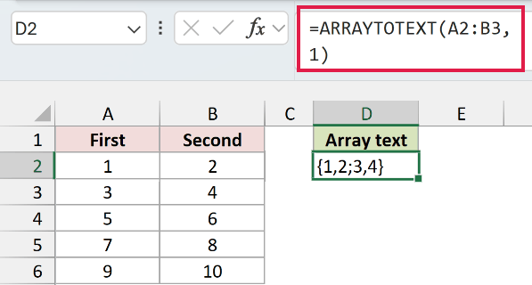
The text result is {1,2;3,4}.

VALUETOTEXT

VALUETOTEXT converts any value to text. In strict mode, text values get wrapped in quotes, so you can tell text apart from numbers.

It’s mostly useful when you’re checking data types or building strings from mixed values, and you want to see exactly what Excel is storing.

Convert a single label to strict text.

=VALUETOTEXT(A2,1)

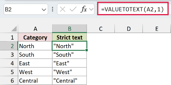
The North label appears as quoted text.

TEXTAFTER

TEXTAFTER returns everything that comes after a character or word you choose. Give it a hyphen, and it hands back whatever follows the hyphen.

It’s much simpler than the old MID and FIND combination. You can also pick which occurrence to use, like the text after the second comma.

Return the part of each shipment code after the hyphen.

=TEXTAFTER(A2:A7,"-")

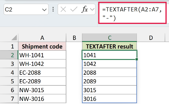
WH-1041 becomes 1041.

TEXTBEFORE

TEXTBEFORE is the opposite of TEXTAFTER. It returns everything that comes before the character or word you choose.

Use it to grab first names, email usernames, product prefixes, or anything else that sits at the start of a text string.

Return the part of each shipment code before the hyphen.

=TEXTBEFORE(A2:A7,"-")

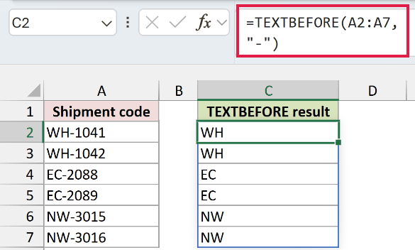
WH-1041 becomes WH.

TEXTSPLIT

TEXTSPLIT breaks text into separate cells based on a delimiter, like a comma or a space. It’s Text to Columns, but as a formula.

It can split across columns, down rows, or both at once. And since it’s a formula, the result updates whenever the original text changes.

Split a pipe-delimited, comma-separated order record into a grid.

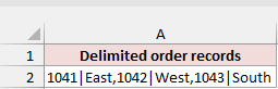
=TEXTSPLIT(A2,"|",",")

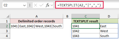
The record becomes rows and columns of order IDs and regions.

Array Reshaping Functions

These functions combine, select, or rearrange ranges. Their results spill, so leave the destination cells empty.

VSTACK

VSTACK stacks ranges on top of each other into one list. Give it two or more ranges, and it puts them one below the other.

It’s perfect for combining data from different sheets or months into a single table, without any copying and pasting.

Put the May name-and-units range below the April range.

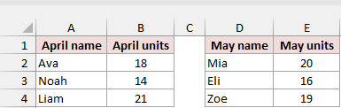
=VSTACK(A2:B4,D2:E4)

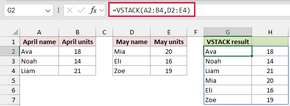
The result is one six-row list.

HSTACK

HSTACK is the side-by-side version of VSTACK. It places ranges next to each other, from left to right.

Use it to pull columns from different places into one table, or to put columns in a different order than the source.

Place units sold beside the product names.

=HSTACK(A2:A7,C2:C7)

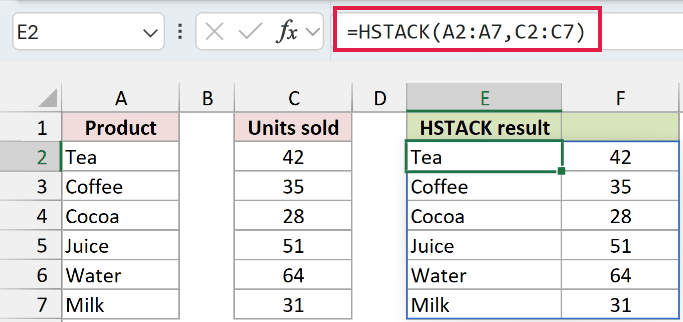
A two-column product-and-units array spills.

TOROW

TOROW takes a range of any shape and flattens it into a single row.

It can also skip blanks or errors along the way, which makes it useful for turning a messy range into one tidy line.

Flatten a two-column color-and-size range across one row.

=TOROW(A2:B4)

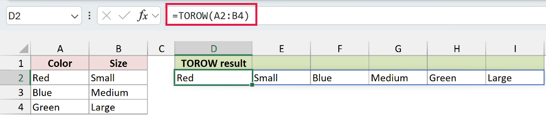
The values spill horizontally in source order.

TOCOL

TOCOL does the same thing as TOROW, but it flattens everything into a single column instead.

It’s the one I use more often, since lists usually run down a column. It’s great for turning a grid into one long list you can sort or filter.

Flatten that range down one column.

=TOCOL(A2:B4)

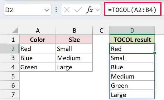
The values spill vertically in source order.

CHOOSECOLS

CHOOSECOLS returns only the columns you pick from a range. You list the column numbers, and it gives you just those.

It’s handy when a table has ten columns but your report only needs two of them. You can pick them in any order, too.

Keep the first and fourth columns from the employee table.

=CHOOSECOLS(A1:D7,1,4)

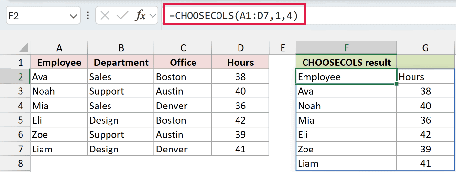
The result shows employees and hours.

CHOOSEROWS

CHOOSEROWS works the same way, but for rows. You list the row numbers you want, and it returns only those rows.

Use a negative number to count from the bottom, which is a nice way to grab the last row of a list.

Keep selected rows from the route list.

=CHOOSEROWS(A1:B7,1,3,5,7)

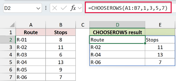
The header and three selected route records spill.

DROP

DROP removes a set number of rows or columns from the start or end of a range, and returns what’s left.

The most common use is dropping a header row. Use a negative number to drop from the end instead, like removing a totals row.

Remove the first row from the ticket range.

=DROP(A1:C7,1)

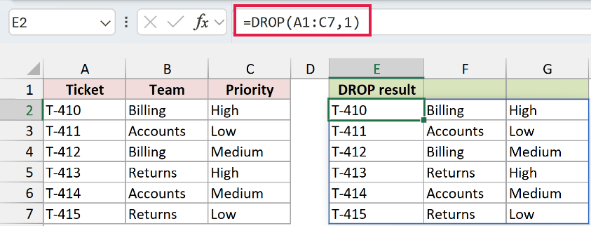
The ticket data remains without its header.

EXPAND

EXPAND makes a range bigger by adding extra rows or columns. You choose the new size and what to fill the new cells with.

Without a fill value, the new cells show #N/A. It’s mostly useful when you need two arrays to be the same size before you stack or combine them.

Grow a weekly-orders range to five rows and four columns.

=EXPAND(A1:B5,5,4,"—")

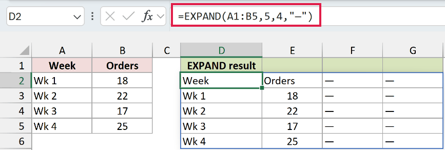
New cells receive the specified dash filler.

TAKE

TAKE is the opposite of DROP. Instead of removing rows or columns, it keeps only the number you ask for from the start or end.

It’s great for top-N lists. Sort your data, then TAKE the first five rows. Or use a negative number to get the last few entries.

Return the last three rows from the sales range.

=TAKE(A1:C7,-3)

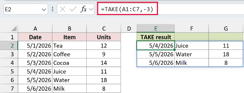
Only the last three records spill.

WRAPCOLS

WRAPCOLS takes a single list and wraps it into columns of a set length. Once a column fills up, it starts the next one.

It’s useful for turning a long list into a more compact layout, like splitting 30 names into three columns of 10.

Wrap a six-item training list into columns with three items each.

=WRAPCOLS(A2:A7,3,"")

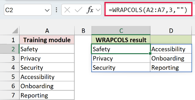
The list becomes a three-row grid.

WRAPROWS

WRAPROWS does the same thing, but it fills across rows instead. Set how many values go in each row, and it wraps the rest.

Use it when data is stuck in one column but actually belongs in a table, like records that repeat every three cells.

Wrap the same six items into rows of three.

=WRAPROWS(A2:A7,3,"")

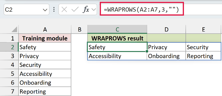
The list becomes a two-row grid.

Summary Functions

Use GROUPBY for totals by one field, PIVOTBY for a cross-tab, and PERCENTOF for one set’s share of another.

GROUPBY

GROUPBY summarizes data by a field you choose. Give it the column to group by, the values, and a function like SUM or AVERAGE.

You get pivot-table-style totals from a single formula. And unlike a pivot table, it updates automatically when the data changes, with no Refresh needed.

Sum museum tickets sold by gallery.

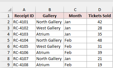
=GROUPBY(B2:B9,D2:D9,SUM,0,0)

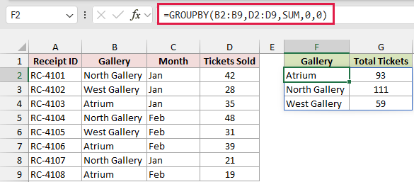
The result spills one total per gallery.

PIVOTBY

PIVOTBY builds a full cross-tab with one formula. You pick what goes in the rows, what goes in the columns, and what to summarize.

It’s like a pivot table you never have to refresh. Use it when you need totals broken down two ways, like sales by region and by month.

PIVOTBY cross-tabs tickets sold by gallery and month.

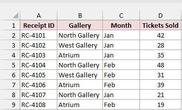
=PIVOTBY(B2:B9,C2:C9,D2:D9,SUM,0,0,,0)

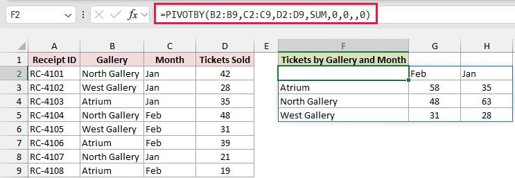
The result spills gallery rows, month columns, and their totals.

PERCENTOF

PERCENTOF works out what share one set of values is of a bigger total. It adds up the subset and divides it by the sum of the whole range.

It saves you from writing SUM divided by SUM, and it works well inside GROUPBY and PIVOTBY for showing percentages of a total.

Calculate the first two galleries’ tickets as a share of all five.

=PERCENTOF(B2:B3,B2:B6)

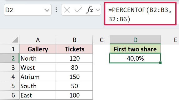
The result is 40%.

Regex Functions and TRIMRANGE

Regex formulas test, extract, or replace a text pattern. TRIMRANGE removes blank outer edges from a range.

REGEXTEST

REGEXTEST checks whether text matches a pattern and returns TRUE or FALSE. The pattern uses regular expressions, a short code for describing what text should look like.

It’s great for validating things like IDs, email addresses, or phone numbers, where you care about the format rather than an exact value.

Check whether a booking ID fits the BK-#### pattern.

=REGEXTEST(A2,"^BK-[0-9]{4}$")

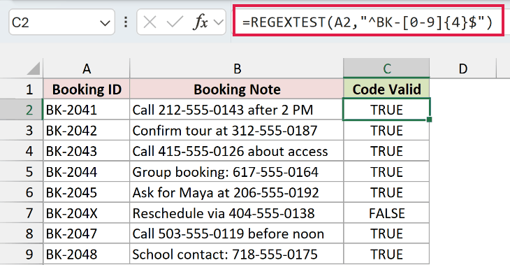
The valid sample ID returns TRUE.

REGEXEXTRACT

REGEXEXTRACT pulls out the part of a text string that matches a pattern. You describe what you’re looking for, and it finds it.

Use it to grab phone numbers, order IDs, or dates from messy notes, even when they sit in a different place in every cell.

Pull a phone number from a booking note.

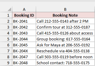
=REGEXEXTRACT(B2,"[0-9]{3}-[0-9]{3}-[0-9]{4}")

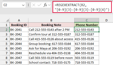
The first note returns 212-555-0143.

REGEXREPLACE

REGEXREPLACE finds text that matches a pattern and swaps it for something else.

It’s like Find and Replace, but much smarter. You can mask every phone number or fix inconsistent formats in one go, without knowing the exact text in advance.

Mask phone numbers inside booking notes.

=REGEXREPLACE(B2,"[0-9]{3}-[0-9]{3}-[0-9]{4}","XXX-XXX-XXXX")

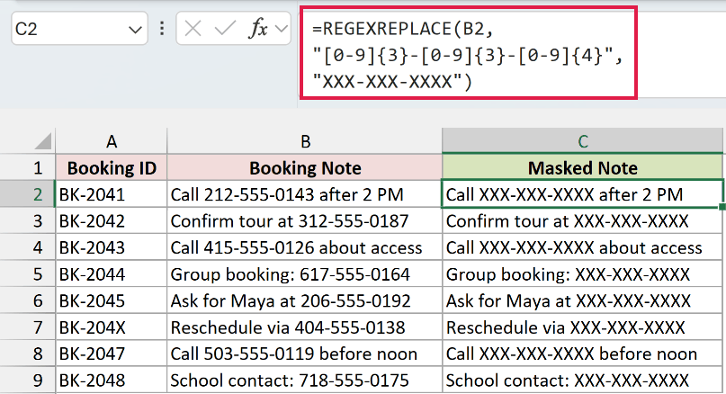
The first phone number becomes XXX-XXX-XXXX.

TRIMRANGE

TRIMRANGE removes empty rows and columns from the edges of a range. You get back only the part that actually has data.

It’s useful when you point a formula at a big range so new data gets picked up, but you don’t want hundreds of blank rows in the result.

Remove blank rows and columns around a pasted museum export.

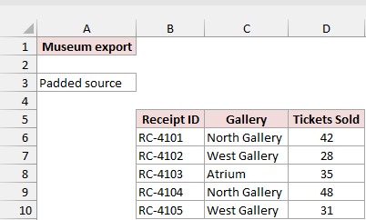
=TRIMRANGE(A4:D13)

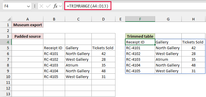
The meaningful table remains as a spill range.

Connected Functions (Need Internet)

These four pull data, images, or translations from outside your workbook, so they need an internet connection. That’s why the download shows their formulas as text instead of live results.

STOCKHISTORY

STOCKHISTORY pulls historical price data for a stock, fund, or currency straight into Excel. You give it a ticker symbol and a date range.

You can choose daily, weekly, or monthly data, and which columns to show, like the close, open, high, low, or volume.

Request daily dates and closing prices for MSFT over January 4–8, 2021.

=STOCKHISTORY("MSFT",DATE(2021,1,4),DATE(2021,1,8),0,1,0,1)

In a connected copy of Excel, this returns the dates and closing prices for those five days.

IMAGE

IMAGE puts a picture from the web right inside a cell. You give it the image URL, plus optional alt text and sizing.

The picture stays in its cell when you sort, filter, or resize, which makes it great for product lists and catalogs. The image needs an HTTPS web address.

Place a company logo from an HTTPS URL in a cell.

=IMAGE("https://example.com/logo.png","Company logo")

The URL is just a placeholder, so swap in a real image address.

TRANSLATE

TRANSLATE converts text from one language to another, right in a cell. You give it the text and the language to translate into.

Excel can detect the source language for you, but it’s more reliable to specify it, especially for short text. It’s handy for product names, feedback, or quick notes.

Translate Hello from English to Spanish through the online service.

=TRANSLATE(A2,"en","es")

In a connected copy of Excel, this returns Hola.

DETECTLANGUAGE

DETECTLANGUAGE tells you which language a piece of text is written in. It returns a short language code, like es for Spanish.

Pair it with TRANSLATE when you have mixed-language data and need to know what you’re working with first.

Identify the language of Bonjour through the online service.

=DETECTLANGUAGE(A2)

In a connected copy of Excel, this returns fr, the language code for French.

Additional Notes About New Excel Functions

• A dynamic array needs clear cells for its spill range. A blocked cell can cause #SPILL!.
• Some formulas recalculate when their inputs change. RANDARRAY also changes on recalculation, so its exact numbers are not fixed.
• Function availability varies by Excel version, update channel, and platform. #NAME? often means your installation does not recognize the function.
• STOCKHISTORY, IMAGE, TRANSLATE, and DETECTLANGUAGE require connected data or reachable content. The download labels these four as reference examples.
• GROUPBY and PIVOTBY are formulas that return summary arrays. A PivotTable is a separate interactive Excel feature.

Frequently Asked Questions

Why does a formula show #NAME? on my computer?

Your Excel build may not include that function yet, or it may be unavailable on your platform or update channel.

Check File > Account > Update Options and the linked Microsoft support page.

Do any of these work in Excel 2021 or Excel 2024?

Yes. Some later perpetual releases include selected functions from this list.

Check the version badges on each function’s Microsoft support page rather than assuming that every Microsoft 365 function is included.

Why does a formula spill into other cells?

Functions such as FILTER and VSTACK return arrays. Excel displays their results across as many cells as needed. Clear any existing contents in that destination area if you get #SPILL!.

Which examples need an internet connection or service?

STOCKHISTORY, IMAGE, TRANSLATE, and DETECTLANGUAGE depend on external data, images, or Microsoft’s connected services. The download keeps their formulas as readable references.

How are GROUPBY and PIVOTBY different from a PivotTable?

GROUPBY and PIVOTBY return dynamic formula results. PivotTables use Excel’s separate pivot interface and refresh controls. Choose according to how you want to edit and present the summary.

Conclusion

That’s all 44, and you don’t need to learn them all at once.

Pick a task you already do in Excel, find the matching function here, and try it on its example sheet first.

I hope you found this article helpful.